38 excel chart only show certain data labels

Add or remove data labels in a chart - support.microsoft.com Click the data series or chart. To label one data point, after clicking the series, click that data point. In the upper right corner, next to the chart, click Add Chart Element > Data Labels. To change the location, click the arrow, and choose an option. If you want to show your data label inside a text bubble shape, click Data Callout. How to make a chart (graph) in Excel and save it as template 22/10/2015 · 3. Inset the chart in Excel worksheet. To add the graph on the current sheet, go to the Insert tab > Charts group, and click on a chart type you would like to create.. In Excel 2013 and Excel 2016, you can click the Recommended Charts button to view a gallery of pre-configured graphs that best match the selected data.. In this example, we are creating a 3-D …

peltiertech.com › cusCustom Axis Labels and Gridlines in an Excel Chart Jul 23, 2013 · Select the vertical dummy series and add data labels, as follows. In Excel 2007-2010, go to the Chart Tools > Layout tab > Data Labels > More Data label Options. In Excel 2013, click the “+” icon to the top right of the chart, click the right arrow next to Data Labels, and choose More Options….

Excel chart only show certain data labels

Is there a way to show only specific values in x-axis of an excel chart ... 1) Use a line chart, which treats the horizontal axis as categories (rather than quantities). 2) Use an XY/Scatter plot, with the default horizontal axis "turned off" and replaced with a "helper" series with vertical values of 0 and horizontal values as desired in your dataset (this is my preferred method). EDIT: Step by Step directions, Only Display Some Labels On Pie Chart - Excel Help Forum For a new thread (1st post), scroll to Manage Attachments, otherwise scroll down to GO ADVANCED, click, and then scroll down to MANAGE ATTACHMENTS and click again. Now follow the instructions at the top of that screen. New Notice for experts and gurus: Display every "n" th data label in graphs - Microsoft Community you can use a free tool created by Rob Bovey, called the XY Chart Labeler. With this tool you can assign a range of cells to be the labels for chart series, instead of the Excel defaults. Using a formula, you can have a text show up in every nth cell and then use that range with the XY Chart Labeler to display as the series label.

Excel chart only show certain data labels. How to Change Excel Chart Data Labels to Custom Values? - Chandoo.org First add data labels to the chart (Layout Ribbon > Data Labels) Define the new data label values in a bunch of cells, like this: Now, click on any data label. This will select "all" data labels. Now click once again. At this point excel will select only one data label. Go to Formula bar, press = and point to the cell where the data label ... How to create Custom Data Labels in Excel Charts - Efficiency 365 Create the chart as usual. Add default data labels. Click on each unwanted label (using slow double click) and delete it. Select each item where you want the custom label one at a time. Press F2 to move focus to the Formula editing box. Type the equal to sign. Now click on the cell which contains the appropriate label. PowerPoint: Where’s My Chart Data? – IT Training Tips - IU 17/03/2011 · HI, I am using Excel 2007 and have created hundreds of charts which are copied into PowerPoint (and linked) but when I update the data in Excel the changes are not reflected in PowerPoint. However, if I make the changes in PowerPoint by editing the data on each chart the changes are reflected in the original Excel file. I need a quicker way to ... Excel chart not showing all data selected - Microsoft Community Double-click any of the dates along the x-axis, or the x-axis itself. In the Format Axis taskpane, look at the Minimum and Maximum. If you see Reset next to the box, click it to make the bound automatic (it should read Auto after that) ---, Kind regards, HansV, , Report abuse, 88 people found this reply helpful, ·,

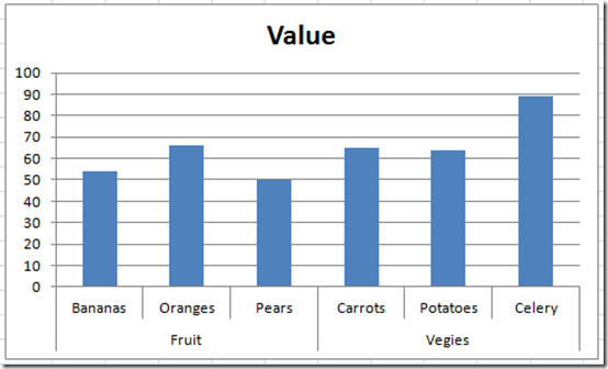
How can I hide 0% value in data labels in an Excel Bar Chart The quick and easy way to accomplish this is to custom format your data label. Select a data label. Right click and select Format Data Labels; Choose the Number category in the Format Data Labels dialog box. Data Analysis in Excel (In Easy Steps) - Excel Easy 9 Data Form: The data form in Excel allows you to add, edit and delete records (rows) and display only those records that meet certain ... Use a bar chart if you have large text labels. To create a bar chart in Excel, execute the following steps. 28 Area Chart: An area chart is a line chart with the areas below the lines filled with colors. Use a stacked area chart to display the … excelmate.wordpress.com › 2014/07/15 › 637Excel – Create a Dynamic 12 Month Rolling Chart | Excelmate Jul 15, 2014 · To create a dynamic chart using this simple table we will need two named dynamic ranges – one for the data itself and one for the labels. Note that when working with charts you will need to create a separate dynamic range for each series as charts treat each series separately so you cannot create a single dynamic named range that includes all rows and columns. Find, label and highlight a certain data point in Excel scatter graph 10/10/2018 · Click the Chart Elements button. Select the Data Labels box and choose where to position the label. By default, Excel shows one numeric value for the label, y value in our case. To display both x and y values, right-click the label, click Format Data Labels…, select the X Value and Y value boxes, and set the Separator of your choosing:

Data Labels - I Only Want One - Google Groups Use ribbon Chart Tools >, Layout > Labels > Data Labels > More Data Label Options. You can now apply specific label type to selected point only. Another way would be to add a dummy series that only... Label Specific Excel Chart Axis Dates • My Online Training Hub Steps to Label Specific Excel Chart Axis Dates. The trick here is to use labels for the horizontal date axis. We want these labels to sit below the zero position in the chart and we do this by adding a series to the chart with a value of zero for each date, as you can see below: Note: if your chart has negative values then set the 'Date Label ... › how-to-create-excel-pie-chartsHow to Make a Pie Chart in Excel & Add Rich Data Labels to ... Sep 08, 2022 · 3) Select the Unforced Errors data point only, (the currently orange shaded data point), since we now only want to format this particular data point with specific formatting. 4) Go to Chart Tools>Format>Shape Styles>Click on the drop-down next to Shape Fill and select More Fill Colors. Highlight a Specific Data Label in an Excel Chart - Peltier Tech * right click on the series, choose Change Series Chart Type from the pop up menu, and select the desired chart type. Add data labels to each line chart* (left), then format them as desired (right). * right click on the series, choose Add Data Labels from the pop up menu. Finally format the two line chart series so they use no line and no marker.

Display Data Labels for only the First and Last Data Points Basically, I want to get rid of the center labels for the red and blue lines (series). This is a dynamic graph and the value will vary by user input. Thus, I can't simply delete these labels and fix the problem. I need to set-up excel so that only the first and last values of the two series have labels. The end result would look like:

How to Make a Pie Chart in Excel & Add Rich Data Labels to The Chart! 08/09/2022 · A pie chart is used to showcase parts of a whole or the proportions of a whole. There should be about five pieces in a pie chart if there are too many slices, then it’s best to use another type of chart or a pie of pie chart in order to showcase the data better. In this article, we are going to see a detailed description of how to make a pie chart in excel.

› make-graph-excel-chart-templateHow to make a chart (graph) in Excel and save it as template Oct 22, 2015 · 11 comments to "How to create a chart (graph) in Excel and save it as template" Amit says: May 4, 2021 at 4:15 am Hi, When I save the chart as a Template and reuse the template, I cant seem to get the custom data labels from the original chart. Is there a special way to do this. Thanks. Reply; Robert NP says: March 5, 2020 at 7:55 pm

› office-addins-blog › 2018/10/10Find, label and highlight a certain data point in Excel ... Oct 10, 2018 · Click the Chart Elements button. Select the Data Labels box and choose where to position the label. By default, Excel shows one numeric value for the label, y value in our case. To display both x and y values, right-click the label, click Format Data Labels…, select the X Value and Y value boxes, and set the Separator of your choosing:

charts - Excel, giving data labels to only the top/bottom X% values ... 1) Create a data set next to your original series column with only the values you want labels for (again, this can be formula driven to only select the top / bottom n values). See column D below. 2) Add this data series to the chart and show the data labels. 3) Set the line color to No Line, so that it does not appear! 4) Volia! See Below! Share,

Add a DATA LABEL to ONE POINT on a chart in Excel Steps shown in the video above: Click on the chart line to add the data point to. All the data points will be highlighted. Click again on the single point that you want to add a data label to. Right-click and select ' Add data label ', This is the key step! Right-click again on the data point itself (not the label) and select ' Format data label '.

Hiding data labels for some, not all values in a series Here's a good challenge for you. I can't figure it out, and I believe it's a limitation of Excel. I have a bar graph with several data series. I know how to show the data labels for every data point in a given series. But I'm looking to show the data label for only some data points in a given series -- i.e. non-zero valued data points.

Excel tutorial: How to use data labels In this video, we'll cover the basics of data labels. Data labels are used to display source data in a chart directly. They normally come from the source data, but they can include other values as well, as we'll see in in a moment. Generally, the easiest way to show data labels to use the chart elements menu. When you check the box, you'll see ...

Add data labels and callouts to charts in Excel 365 - EasyTweaks.com The steps that I will share in this guide apply to Excel 2021 / 2019 / 2016. Step #1: After generating the chart in Excel, right-click anywhere within the chart and select Add labels . Note that you can also select the very handy option of Adding data Callouts.

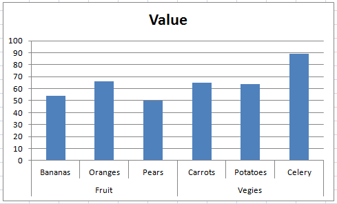
Add / Move Data Labels in Charts - Excel & Google Sheets Check Data Labels . Change Position of Data Labels. Click on the arrow next to Data Labels to change the position of where the labels are in relation to the bar chart. Final Graph with Data Labels. After moving the data labels to the Center in this example, the graph is able to give more information about each of the X Axis Series.

Only chart certain values - Excel Help Forum Have the data you are pulling from be the result of formulas such as, =IF (xyz=0,NA (),xyz) This means that in place of 0 you will have N/A and that will not be plotted, on the chart (Unless it is one specific type which will still show it -, Can't remember which). Assume it's a line chart or something similar and you just don't want the,

How to Only Show Selected Data Points in an Excel Chart Download Free Sample Dashboard Files here: on how to show or hide specific data points i...

How to Conditionally Show or Hide Charts - Excel Chart Templates ... The Solution: Use INDIRECT () and a nifty image hack. First, create your charts in a separate worksheet like this (remember you need to create all 3 charts first) Once the charts are created adjust the width and heights of 3 cells and place one chart in each like above. Now, go back to the sheet where you want to control the display, and define ...

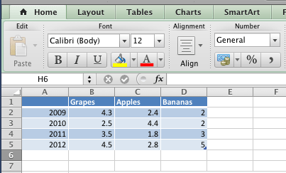
How to Use Cell Values for Excel Chart Labels - How-To Geek Select the chart, choose the "Chart Elements" option, click the "Data Labels" arrow, and then "More Options.". Uncheck the "Value" box and check the "Value From Cells" box. Select cells C2:C6 to use for the data label range and then click the "OK" button. The values from these cells are now used for the chart data labels.

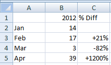
Excel tutorial: Dynamic min and max data labels To make the formula easy to read and enter, I'll name the sales numbers "amounts". The formula I need is: =IF (C5=MAX (amounts), C5,"") When I copy this formula down the column, only the maximum value is returned. And back in the chart, we now have a data label that shows maximum value. Now I need to extend the formula to handle the minimum value.

Excel Chart not showing SOME X-axis labels - Super User 05/04/2017 · I have a chart that refreshes after a dataload, and it seems like when there are more than 25 labels on the x-axis, the 26th and on do not show, though all preceding values do. Also, the datapoints for those values show in the chart. In the chart data window, the labels are blank.

Only Label Specific Dates in Excel Chart Axis - YouTube Date axes can get cluttered when your data spans a large date range. Use this easy technique to only label specific dates.Download the Excel file here: https...

Share :