43 excel chart change labels
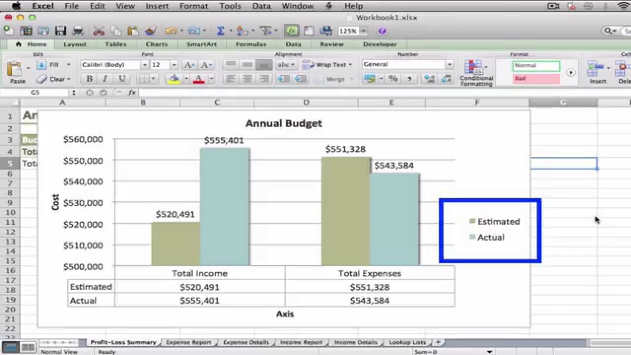
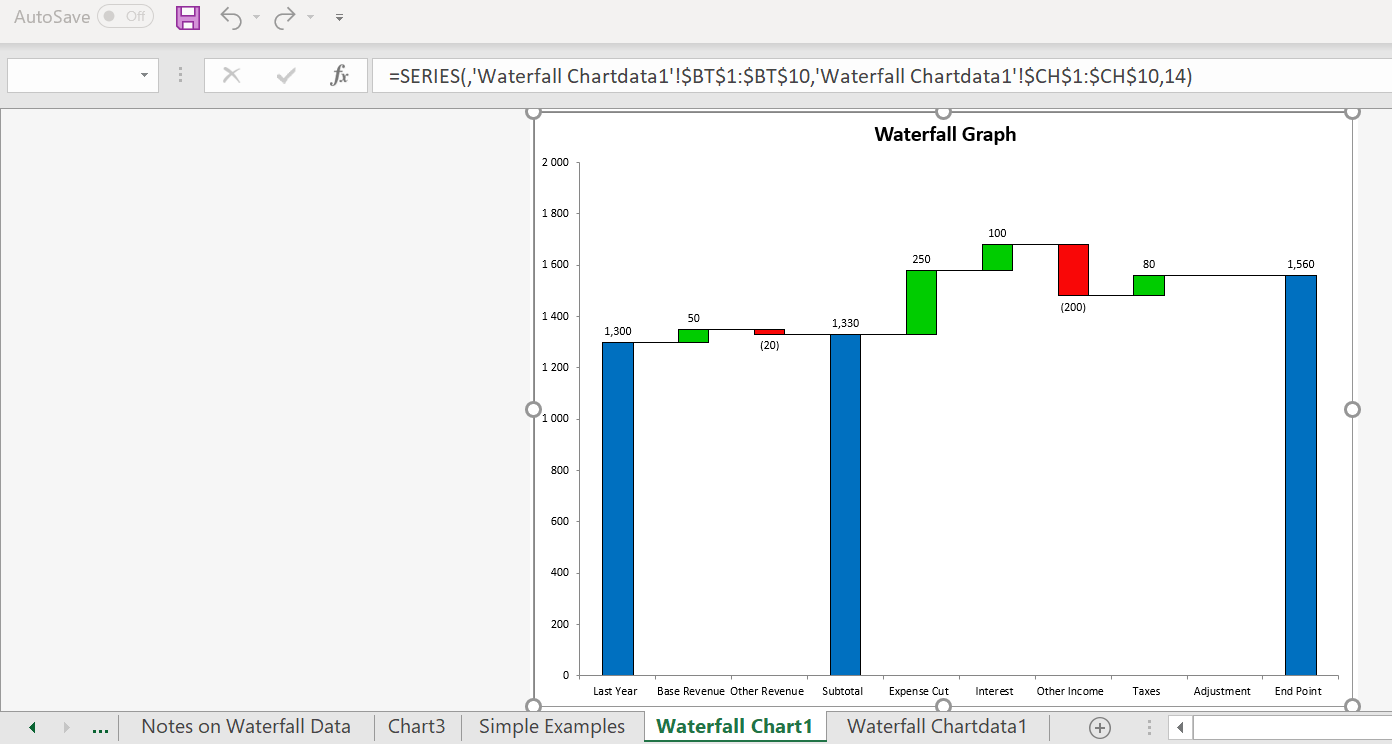
How to Create and Customize a Waterfall Chart in Microsoft Excel Select the chart and use the buttons on the right (Excel on Windows) to adjust Chart Elements like labels and the legend, or Chart Styles to pick a theme or color scheme. Select the chart and go to the Chart Design tab. How to add text labels on Excel scatter chart axis Add dummy series to the scatter plot and add data labels. 4. Select recently added labels and press Ctrl + 1 to edit them. Add custom data labels from the column "X axis labels". Use "Values from Cells" like in this other post and remove values related to the actual dummy series. Change the label position below data points.
Excel charts: Labels on X-axis start at the wrong value EDIT: Further explanation based on the comment You need to explicitly select the x-axis by clicking on it so that it is highlighted as shown below (not the yellow part of course): If this does not work, you can also select the x-axis in the following way; assuming you are able to adjust the y-axis as mentioned in your comment.
Excel chart change labels
All About Chart Elements in Excel - Add, Delete, Change - Excel Unlocked By default, Excel writes the text string "Chart Title" at the place of the chart title. We can rename the chart title by double-clicking on it. i.e "Monthly Sales" We can also change the position of the chart title by simply dragging it using the cursor. Download Above Image to Your Desktop >>>> Download Chart Data Labels How to make shading on Excel chart and move x axis labels to the bottom ... In the Change Chart Type dialog, change the chart type for the new series to Stacked Area. Change the color from whatever Excel decides to yellow. Finally, remove the new series form the legend. See the attached version. Wi-Fi Signal Strength.xlsx 15 KB 0 Likes Reply Snoopdon replied to Hans Vogelaar Oct 24 2021 05:18 PM Excel: How to Create a Bubble Chart with Labels - Statology Step 3: Add Labels. To add labels to the bubble chart, click anywhere on the chart and then click the green plus "+" sign in the top right corner. Then click the arrow next to Data Labels and then click More Options in the dropdown menu: In the panel that appears on the right side of the screen, check the box next to Value From Cells within ...
Excel chart change labels. How to Edit Pie Chart in Excel (All Possible Modifications) Just like the chart title, you can also change the position of data labels in a pie chart. Follow the steps below to do this. 👇 Steps: Firstly, click on the chart area. Following, click on the Chart Elements icon. Subsequently, click on the rightward arrow situated on the right side of the Data Labels option. TickLabels object (Excel Graph) | Microsoft Docs To change the tick-mark label text for the value axis, you must change the values of these properties. Use the TickLabels property to return the TickLabels object. Example. The following example sets the number format for the tick-mark labels on the value axis in the chart. myChart.Axes(xlValue).TickLabels.NumberFormat = "0.00" See also How to Change the Y Axis in Excel - Alphr Click the dropdown next to "Display Units," then make your selection such as "millions" or "hundreds." To label the displayed units, go to the "Axis Options -> Display units" section. Add a... How to format axis labels individually in Excel - SpreadsheetWeb Double-click on the axis you want to format. Double-clicking opens the right panel where you can format your axis. Open the Axis Options section if it isn't active. You can find the number formatting selection under Number section. Select Custom item in the Category list. Type your code into the Format Code box and click Add button.
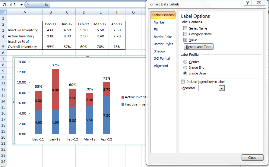
How to Show Pie Chart Data Labels in Percentage in Excel Nothing, we'll just change the chart design to a specific design that has built-in percentage data labels in it. Steps: Select the chart by clicking anywhere on it. Next, click on the Chart Styles icon. Then select a chart style from the appeared list that has percentage labels. I selected Style 3. You can do the same thing using another way. Chart.ApplyDataLabels method (Excel) | Microsoft Docs The type of data label to apply. True to show the legend key next to the point. The default value is False. True if the object automatically generates appropriate text based on content. For the Chart and Series objects, True if the series has leader lines. Pass a Boolean value to enable or disable the series name for the data label. How to Add Labels to Scatterplot Points in Excel - Statology Step 3: Add Labels to Points Next, click anywhere on the chart until a green plus (+) sign appears in the top right corner. Then click Data Labels, then click More Options… In the Format Data Labels window that appears on the right of the screen, uncheck the box next to Y Value and check the box next to Value From Cells. Modifying Axis Scale Labels (Microsoft Excel) Follow these steps: Create your chart as you normally would. Double-click the axis you want to scale. You should see the Format Axis dialog box. (If double-clicking doesn't work, right-click the axis and choose Format Axis from the resulting Context menu.) Make sure the Number tab is displayed. (See Figure 1.) Figure 1.
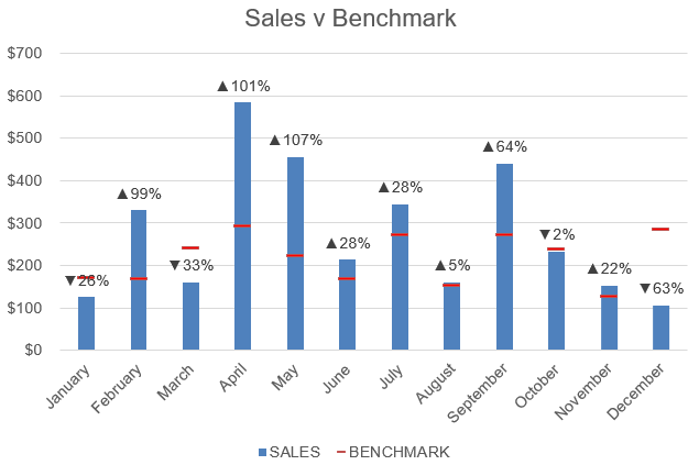
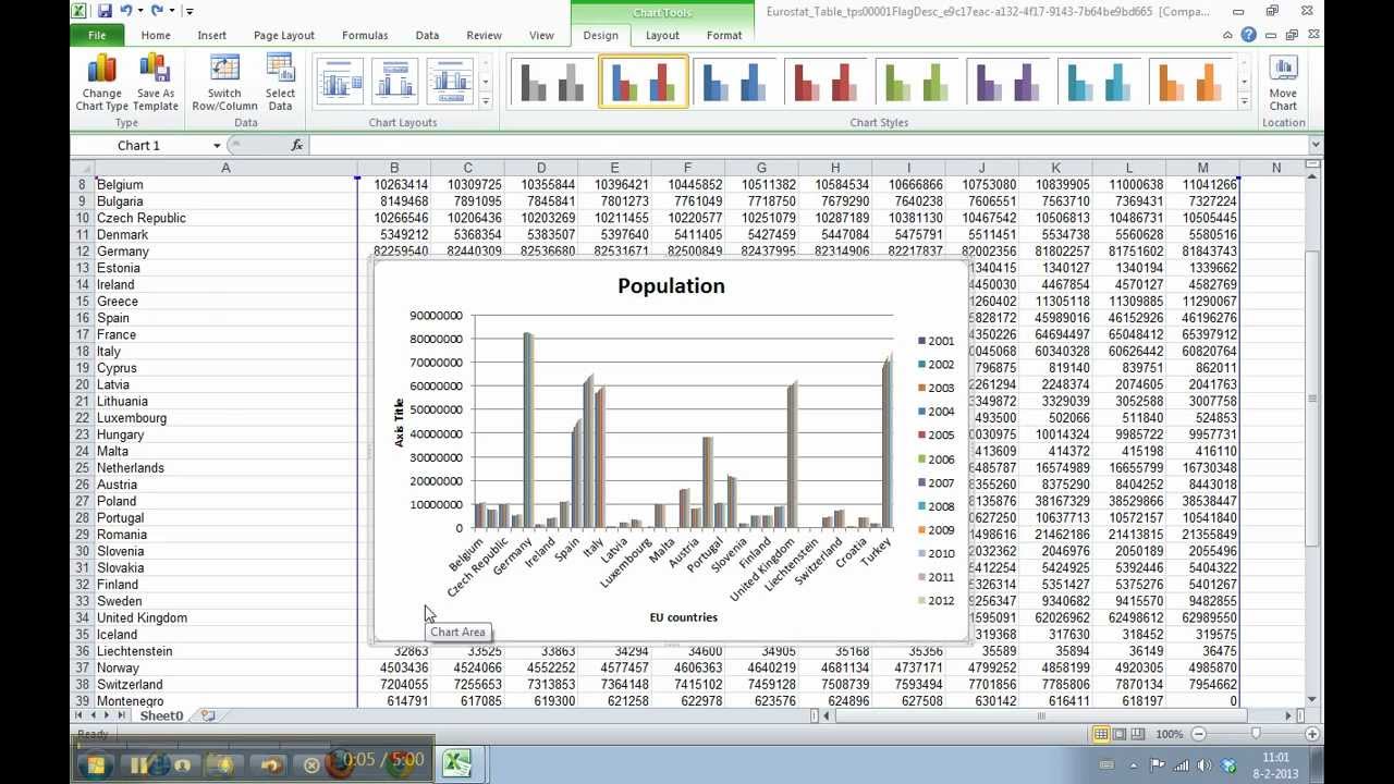
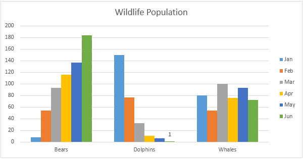
Horizontal axis labels on a chart - Microsoft Community Fill a range of 12 cells with the months of the year. If you start with Jan or January, then fill down, Excel should automatically fill in the following names. Click on the chart. Click 'Select Data' on the 'Chart Design' tab of the ribbon. Click Edit under 'Horizontal (Category) Axis Labels'. Point to the range with the months, then OK your ... How to Add Total Values to Stacked Bar Chart in Excel Step 4: Add Total Values. Next, right click on the yellow line and click Add Data Labels. Next, double click on any of the labels. In the new panel that appears, check the button next to Above for the Label Position: Next, double click on the yellow line in the chart. In the new panel that appears, check the button next to No line: How to Print Labels from Excel - Lifewire Select Mailings > Write & Insert Fields > Update Labels . Once you have the Excel spreadsheet and the Word document set up, you can merge the information and print your labels. Click Finish & Merge in the Finish group on the Mailings tab. Click Edit Individual Documents to preview how your printed labels will appear. Select All > OK . How to change the orientation of all chart column labels simultaneously ... Add the labels and set the rotation as you desire. Select the entire chart you just created. Ctrl-C. Select the chart that contains all the series and remove all data labels. On the Home ribbon, press Paste, Paste Special..., Formats. The chart should now have labels in the same orientation for all series.
Position Chart Legend & Display Gridlines in Microsoft Excel: MOOC - YouTube
Excel Area Chart Data Label & Position - ExcelDemy Download Practice Workbook. What Is Area Chart? How to Insert Excel Area Chart Data Label and Change Their Position. 📌 Step 1: Organize Data. 📌 Step 2: Insert Area Chart. 📌 Step 3: Show Data Labels. 📌 Step 4: Format Data Labels. 📌 Step 5: Change Data Label Position. Things to Remember.
Custom Chart Labels Using Excel 2013 | MyExcelOnline
Custom Chart Data Labels In Excel With Formulas Follow the steps below to create the custom data labels. Select the chart label you want to change. In the formula-bar hit = (equals), select the cell reference containing your chart label's data. In this case, the first label is in cell E2. Finally, repeat for all your chart laebls.
How to format the chart axis labels in Excel 2010 - YouTube
How to Change Axis Labels in Excel (3 Easy Methods) To change the label using this method, follow the steps below: Firstly, right-click the category label and click Select Data. Then, click Edit from the Horizontal (Category) Axis Labels icon. After that, assign the new labels separated with commas and click OK. Now, Your new labels are assigned.

Excel 2010 Tutorial Changing Chart Labels Microsoft Training Lesson 21.3 - YouTube
How to change dot label(when I hover mouse on that dot) of - Microsoft ... How to change dot label (when I hover mouse on that dot) of scatter plot. Hello all, I have few queries: 1. Can I edit the text when I hover mouse on dot of scatter plot (chart) 2. Can I use url to redirect to different site. 3. Can I use display image if I hover mouse on the dot.

add labels to excel chart 218253.image0 - Top Label Maker
Change the Font Size, Color, and Style of an Excel Form Control Label For example, if I were to change G2 to a black color and a smaller font, the label would not show these new changes (however, it would change its text if I changed the value in G2 to something else). So to change the Label's formatting — even when it's linked to the same cell — you'll need to click the label, click the formula bar ...
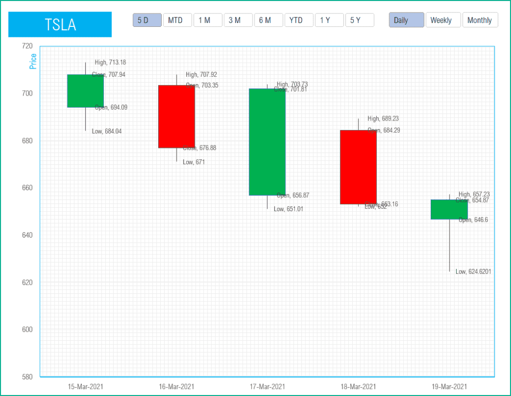
Candlestick Chart Excel Template - Excel for Stock Market
TickLabels object (Excel) | Microsoft Docs Use the TickLabels property of the Axis object to return the TickLabels object. The following example sets the number format for the tick-mark labels on the value axis in embedded chart one on Sheet1. VB Copy Worksheets ("sheet1").ChartObjects (1).Chart _ .Axes (xlValue).TickLabels.NumberFormat = "0.00" Methods Delete Select Properties Alignment
How-to Put Percentage Labels on Top of a Stacked Column Chart - Excel Dashboard Templates
Use defined names to automatically update a chart range - Office On the Insert menu, click Chart to start the Chart Wizard. Click a chart type, and then click Next. Click the Series tab. In the Series list, click Sales. In the Category (X) axis labels box, replace the cell reference with the defined name Date. For example, the formula might be similar to the following: =Sheet1!Date
Charts in Excel - Easy Excel Tutorial
How to Apply a Filter to a Chart in Microsoft Excel Go to the Home tab, click the Sort & Filter drop-down arrow in the ribbon, and choose "Filter.". Click the arrow at the top of the column for the chart data you want to filter. Use the Filter section of the pop-up box to filter by color, condition, or value. When you finish, click "Apply Filter" or check the box for Auto Apply to see ...

31 What Is A Label In Excel - Labels For Your Ideas
Format Chart Axis in Excel - Axis Options Analyzing Format Axis Pane. Right-click on the Vertical Axis of this chart and select the "Format Axis" option from the shortcut menu. This will open up the format axis pane at the right of your excel interface. Thereafter, Axis options and Text options are the two sub panes of the format axis pane.
Waterfall Chart Templates (Excel 2010 and 2013) – Edward Bodmer – Project and Corporate Finance
How to Change Font Size of Data Labels in Excel - ExcelDemy Fourthly, select the whole graph and click on the Chart Elements option and go to the Data Labels. After that, you will get the result like the below image. Next, select the data chart and go to the Home tab. Then, choose the font size accordingly. Finally, the following result will come up on your screen.
Creating a chart with dynamic labels - Microsoft Excel 2016
Excel: How to Create a Bubble Chart with Labels - Statology Step 3: Add Labels. To add labels to the bubble chart, click anywhere on the chart and then click the green plus "+" sign in the top right corner. Then click the arrow next to Data Labels and then click More Options in the dropdown menu: In the panel that appears on the right side of the screen, check the box next to Value From Cells within ...
Excel Charts: Creating Custom Data Labels - YouTube
How to make shading on Excel chart and move x axis labels to the bottom ... In the Change Chart Type dialog, change the chart type for the new series to Stacked Area. Change the color from whatever Excel decides to yellow. Finally, remove the new series form the legend. See the attached version. Wi-Fi Signal Strength.xlsx 15 KB 0 Likes Reply Snoopdon replied to Hans Vogelaar Oct 24 2021 05:18 PM

Excel Chart Elements: Parts of Charts in Excel | ExcelDemy
All About Chart Elements in Excel - Add, Delete, Change - Excel Unlocked By default, Excel writes the text string "Chart Title" at the place of the chart title. We can rename the chart title by double-clicking on it. i.e "Monthly Sales" We can also change the position of the chart title by simply dragging it using the cursor. Download Above Image to Your Desktop >>>> Download Chart Data Labels
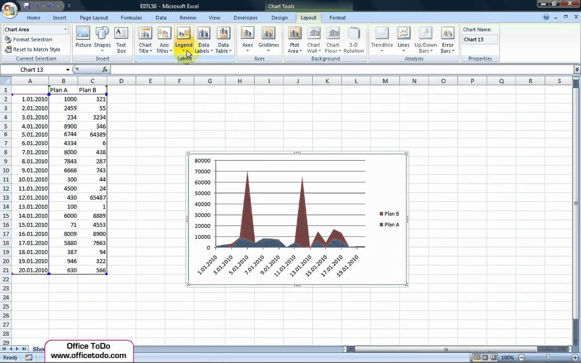
How to add, remove or reposition chart legend? | Excel 2007 - YouTube

Excel Course: Inserting Graphs
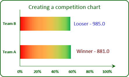
Creating a chart with dynamic labels - Microsoft Excel 2013
Excel Custom Chart Labels • My Online Training Hub
Post a Comment for "43 excel chart change labels"