44 format data labels excel 2016
How to Use Cell Values for Excel Chart Labels - How-To Geek Select the chart, choose the "Chart Elements" option, click the "Data Labels" arrow, and then "More Options.". Uncheck the "Value" box and check the "Value From Cells" box. Select cells C2:C6 to use for the data label range and then click the "OK" button. The values from these cells are now used for the chart data labels. support.microsoft.com › en-us › officeEdit titles or data labels in a chart - support.microsoft.com The first click selects the data labels for the whole data series, and the second click selects the individual data label. Right-click the data label, and then click Format Data Label or Format Data Labels. Click Label Options if it's not selected, and then select the Reset Label Text check box. Top of Page
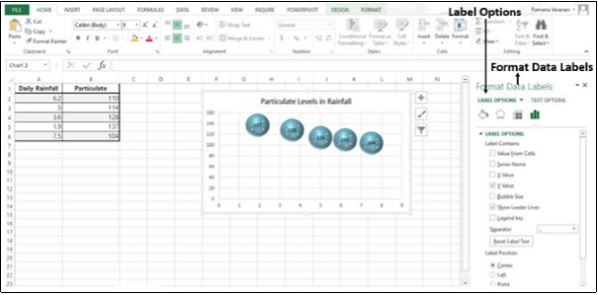
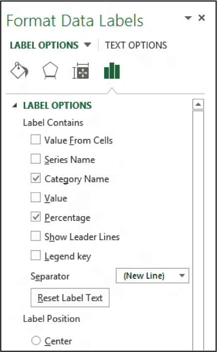
Creating a chart with dynamic labels - Microsoft Excel 2016 1. Right-click on the chart and in the popup menu, select Add Data Labels and again Add Data Labels : 2. Do one of the following: For all labels: on the Format Data Labels pane, in the Label Options, in the Label Contains group, check Value From Cells and then choose cells: For the specific label: double-click on the label value, in the popup ...
Format data labels excel 2016
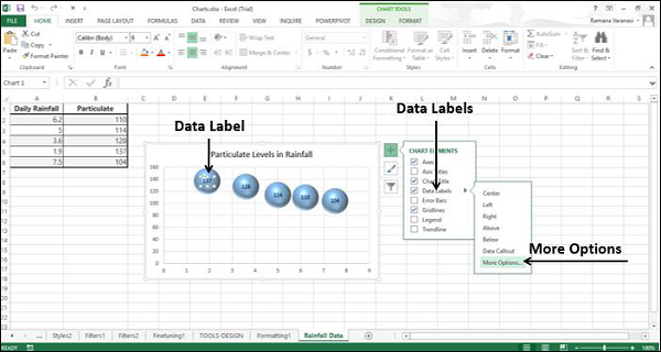
Change Horizontal Axis Values in Excel 2016 - AbsentData 1. Select the Chart that you have created and navigate to the Axis you want to change. 2. Right-click the axis you want to change and navigate to Select Data and the Select Data Source window will pop up, click Edit 3. The Edit Series window will open up, then you can select a series of data that you would like to change. 4. Click Ok Excel Charts: Creating Custom Data Labels - YouTube In this video I'll show you how to add data labels to a chart in Excel and then change the range that the data labels are linked to. This video covers both W... support.microsoft.com › en-us › officeChange the format of data labels in a chart To get there, after adding your data labels, select the data label to format, and then click Chart Elements > Data Labels > More Options. To go to the appropriate area, click one of the four icons ( Fill & Line , Effects , Size & Properties ( Layout & Properties in Outlook or Word), or Label Options ) shown here.
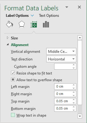
Format data labels excel 2016. Format Data Labels Vertically using Pareto in Excel 2016 Re: Format Data Labels Vertically using Pareto in Excel 2016. Try this: Right-click on one of the data labels > Format Data Labels > Size & Properties > Alignment > Text direction: Stacked. Register To Reply. 10-03-2017, 01:19 PM #3. 1gambit. View Profile. › make-labels-with-excel-4157653How to Print Labels from Excel - Lifewire Choose Start Mail Merge > Labels . Choose the brand in the Label Vendors box and then choose the product number, which is listed on the label package. You can also select New Label if you want to enter custom label dimensions. Click OK when you are ready to proceed. Connect the Worksheet to the Labels › charts › dynamic-chart-dataCreate Dynamic Chart Data Labels with Slicers - Excel Campus Feb 10, 2016 · Step 3: Use the TEXT Function to Format the Labels. Typically a chart will display data labels based on the underlying source data for the chart. In Excel 2013 a new feature called “Value from Cells” was introduced. This feature allows us to specify the a range that we want to use for the labels. › excel_2016 › tipsCreating a simple thermometer chart - Microsoft Excel 2016 Choose the Clustered Column chart.. 3. Remove the horizontal (x) axis.. 4. In the thermometer chart, the column width is equal to the chart width. To make the column occupy the entire width of the plot area, double-click the column to display the Format Data Point task pane (or choose it in the popup menu).
How to Create Mailing Labels in Excel - Excelchat Step 1 - Prepare Address list for making labels in Excel First, we will enter the headings for our list in the manner as seen below. First Name Last Name Street Address City State ZIP Code Figure 2 - Headers for mail merge Tip: Rather than create a single name column, split into small pieces for title, first name, middle name, last name. Move data labels - support.microsoft.com Click any data label once to select all of them, or double-click a specific data label you want to move. Right-click the selection > Chart Elements > Data Labels arrow, and select the placement option you want. Different options are available for different chart types. excel - Change format of all data labels of a single series at once ... A workaround (found prior to #1): A very poor solution, but which possibly saves quite a few keystrokes/mouse clicks in many cases. Select the whole chart, and change the font size in the ribbon. It will change all text. Then recover the font size of all other text but the data labels. 3D maps excel 2016 add data labels Re: 3D maps excel 2016 add data labels. I don't think there are data labels equivalent to that in a standard chart. The bars do have a detailed tool tip but that required the map to be interactive and not a snapped picture. You could add annotation to each point. Select a stack and right click to Add annotation. Cheers.
How to add or move data labels in Excel chart? - ExtendOffice 2. Then click the Chart Elements, and check Data Labels, then you can click the arrow to choose an option about the data labels in the sub menu. See screenshot: In Excel 2010 or 2007. 1. click on the chart to show the Layout tab in the Chart Tools group. See screenshot: 2. Then click Data Labels, and select one type of data labels as you need ... Format Data Labels in Excel- Instructions - TeachUcomp, Inc. To do this, click the "Format" tab within the "Chart Tools" contextual tab in the Ribbon. Then select the data labels to format from the "Chart Elements" drop-down in the "Current Selection" button group. Then click the "Format Selection" button that appears below the drop-down menu in the same area. Excel 2010: How to format ALL data point labels SIMULTANEOUSLY If you want to format all data labels for more than one series, here is one example of a VBA solution: Code: Sub x () Dim objSeries As Series With ActiveChart For Each objSeries In .SeriesCollection With objSeries.Format.Line .Transparency = 0 .Weight = 0.75 .ForeColor.RGB = 0 End With Next End With End Sub. B. Excel 2016: "Value from Cells" box under Format Data Labels Missing 1. The screenshot about the issue. 2. The Office version screenshot via File > Account > Product Information. We will check whether the issue can be reproduced in a specific version. To protect your privacy, please help us mask email address like below: Thanks, Rena ----------------------- * Beware of scammers posting fake support numbers here.
How to create a funny dog breeds lifespan chart in Excel - Microsoft Excel 2016
How to format axis labels as thousands/millions in Excel? 1. Right click at the axis you want to format its labels as thousands/millions, select Format Axis in the context menu. 2. In the Format Axis dialog/pane, click Number tab, then in the Category list box, select Custom, and type [>999999] #,,"M";#,"K" into Format Code text box, and click Add button to add it to Type list. See screenshot: 3.
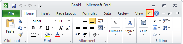
Collapse the Ribbon to get more space on screen - Microsoft Excel 2010
How to Customize Chart Elements in Excel 2016 - dummies In Excel 2016 the Chart Elements button (with the plus sign icon) that appears to the right of an embedded chart when it's selected contains a list of the major chart elements that you can add to your chart. To add an element to your chart, click the Chart Elements button to display an alphabetical list of all the elements, Axes through Trendline. To add a particular element missing ...
Advanced Excel - более богатые метки данных - CoderLessons.com
Conditional formatting of chart axes - Microsoft Excel 2016 To change the format of the label on the Excel 2016 chart axis, do the following: 1. Right-click in the axis and choose Format Axis... in the popup menu: 2. On the Format Axis task pane, in the Number group, select Custom category and then change the field Format Code and click the Add button: If you need a unique representation for positive ...

Sunburst Charts and Treemaps (Excel 2016+) | Microsoft Excel - Dashboards
How to Customize Your Excel Pivot Chart Data Labels - dummies To remove the labels, select the None command. If you want to specify what Excel should use for the data label, choose the More Data Labels Options command from the Data Labels menu. Excel displays the Format Data Labels pane. Check the box that corresponds to the bit of pivot table or Excel table information that you want to use as the label.
Easily create a matrix bubble chart in Excel
Excel 2016 Tutorial Formatting Data Labels Microsoft Training ... - YouTube FREE Course! Click: about Formatting Data Labels in Microsoft Excel at . A clip from Mastering Excel M...

30 What Is A Data Label In Excel - Labels Database 2020
docs.microsoft.com › office-file-format-referenceFile format reference for Word, Excel, and PowerPoint ... Sep 30, 2021 · The macro-enabled file format for an Excel template for Excel 2019, Excel 2016, Excel 2013, Excel 2010, and Office Excel 2007. Stores VBA macro code or Excel 4.0 macro sheets (.xlm). .xltx : Excel Template : The default file format for an Excel template for Excel 2019, Excel 2016, Excel 2013, Excel 2010, and Office Excel 2007.
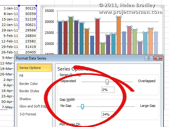
Help! My Excel Chart Columns are too Skinny « projectwoman.com
How do you add data labels to a chart in Excel 2016? To format data labels, select your chart, and then in the Chart Design tab, click Add Chart Element > Data Labels > More Data Label Options. Click Label Options and under Label Contains, pick the options you want. ... To add data labels in Excel 2013 or Excel 2016, follow these steps: Activate the chart by clicking on it, if necessary.

35 Data Label Excel - Labels For Your Ideas
› 07 › 25How to create waterfall chart in Excel 2016, 2013, 2010 ... Jul 25, 2014 · Click on the Base series to select them, right-click and choose the Format Data Series… option from the context menu. The Format Data Series pane immediately appears to the right of your worksheet in Excel 2013 / 2016. Click on the Fill & Line icon. Select No fill in the Fill section and No line in the Border section.
Excel Tips - How to show custom data labels in charts - YouTube
Changing Axis Labels in Excel 2016 for Mac - Microsoft Community In Excel, go to the Excel menu and choose About Excel, confirm the version and build. Please try creating a Scatter chart in a different sheet, see if you are still unable to edit the axis labels; Additionally, please check the following thread for any help" Changing X-axis values in charts. Microsoft Excel for Mac: x-axis formatting. Thanks ...
Format Data Labels in Excel 2013- Tutorial - TeachUcomp, Inc.
Add or remove data labels in a chart - support.microsoft.com Click Label Options and under Label Contains, pick the options you want. Use cell values as data labels You can use cell values as data labels for your chart. Right-click the data series or data label to display more data for, and then click Format Data Labels. Click Label Options and under Label Contains, select the Values From Cells checkbox.

Directly Labeling Excel Charts - Policy Viz
Excel 2016: How to Format Data and Cells - UniversalClass.com To do this, go to the Format Cells dialogue box again, and click Custom n the category column. In the Type list, select the format that you want to customize. As you can see in the snapshot above, we chose the currency format. Now go to the Type field and customize the format by entering the format you want to use. Click OK when you're finished.
30 What Is Data Label In Excel - Labels Design Ideas 2020
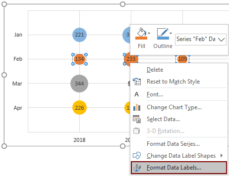
How to create Custom Data Labels in Excel Charts Right click on any data label and choose the callout shape from Change Data Label Shapes option. Now adjust each data label as required to avoid overlap. Put solid fill color in the labels Finally, click on the chart (to deselect the currently selected label) and then click on a data label again (to select all data labels).

Enable or Disable Excel Data Labels at the click of a button - How To - PakAccountants.com
support.microsoft.com › en-us › officeChange the format of data labels in a chart To get there, after adding your data labels, select the data label to format, and then click Chart Elements > Data Labels > More Options. To go to the appropriate area, click one of the four icons ( Fill & Line , Effects , Size & Properties ( Layout & Properties in Outlook or Word), or Label Options ) shown here.

10 Baby Growth Chart Template - Excel Templates
Excel Charts: Creating Custom Data Labels - YouTube In this video I'll show you how to add data labels to a chart in Excel and then change the range that the data labels are linked to. This video covers both W...
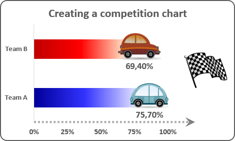
Creating a simple competition chart
Change Horizontal Axis Values in Excel 2016 - AbsentData 1. Select the Chart that you have created and navigate to the Axis you want to change. 2. Right-click the axis you want to change and navigate to Select Data and the Select Data Source window will pop up, click Edit 3. The Edit Series window will open up, then you can select a series of data that you would like to change. 4. Click Ok
Post a Comment for "44 format data labels excel 2016"